Welcome to the DSA Git repository! This repository is dedicated to providing a comprehensive collection of Data Structures and Algorithms implementations and solved coding questions. Whether you’re a beginner or an experienced programmer, this resource aims to support you in enhancing your problem-solving skills and knowledge of DSA concepts.
How to Contribute
We believe in the power of collaboration, and we welcome contributions from the programming community. If you’d like to add new algorithms, optimize existing code, or share your creative problem-solving approaches, follow these steps:
Fork the Repository: Click the “Fork” button on the top right corner of this repository to create your copy.
Clone the Repository: git clone https://github.com/sOR-o/DSA.git
Create a New Branch: git checkout -b feature/new-algorithm
Add Your Code: Add your DSA implementations or coding question solutions to the relevant directories.
Commit and Push: Commit your changes and push them to your forked repository:
git add .
git commit -m "Added new algorithm: XYZ"
git push origin feature/new-algorithm
Create a Pull Request: Go to the original DSA repository on GitHub and click on the “Pull Request” button. Fill in the necessary details and
submit the pull request. Your contribution will be reviewed, and feedback will be provided.
-Can be improved by transfer learning (obviously 😉)
Let’s Learn and Grow Together
We hope this repository becomes a valuable resource in your DSA learning journey. By working together, we can build an ever-expanding collection of DSA implementations and problem-solving insights. Happy coding!
NegMAS is a python library for developing autonomous negotiation agents embedded in simulation environments.
The name negmas stands for either NEGotiation MultiAgent System or NEGotiations Managed by Agent Simulations
(your pick). The main goal of NegMAS is to advance the state of the art in situated simultaneous negotiations.
Nevertheless, it can; and is being used; for modeling simpler bilateral and multi-lateral negotiations, preference elicitation
, etc.
Note
A YouTube playlist to help you use NegMAS for ANAC2020SCM league can be found here
Introduction
This package was designed to help advance the state-of-art in negotiation research by providing an easy-to-use yet
powerful platform for autonomous negotiation targeting situated simultaneous negotiations.
It grew out of the NEC-AIST collaborative laboratory project.
By situated negotiations, we mean those for which utility functions are not pre-ordained by fiat but are a natural
result of a simulated business-like process.
By simultaneous negotiations, we mean sessions of dependent negotiations for which the utility value of an agreement
of one session is affected by what happens in other sessions.
The documentation is available at: documentation (Automatically built versions are available on readthedocs )
Main Features
This platform was designed with both flexibility and scalability in mind. The key features of the NegMAS package are:
The public API is decoupled from internal details allowing for scalable implementations of the same interaction
protocols.
Supports agents engaging in multiple concurrent negotiations.
Provides support for inter-negotiation synchronization either through coupled utility functions or through central
controllers.
Provides sample negotiators that can be used as templates for more complex negotiators.
Supports both mediated and unmediated negotiations.
Supports both bilateral and multilateral negotiations.
Novel negotiation protocols and simulated worlds can be added to the package as easily as adding novel negotiators.
Allows for non-traditional negotiation scenarios including dynamic entry/exit from the negotiation.
A large variety of built in utility functions.
Utility functions can be active dynamic entities which allows the system to model a much wider range of dynamic ufuns
compared with existing packages.
A distributed system with the same interface and industrial-strength implementation is being created allowing agents
developed for NegMAS to be seemingly employed in real-world business operations.
To use negmas in a project
importnegmas
The package was designed for many uses cases. On one extreme, it can be used by an end user who is interested in running
one of the built-in negotiation protocols. On the other extreme, it can be used to develop novel kinds of negotiation
agents, negotiation protocols, multi-agent simulations (usually involving situated negotiations), etc.
In this snippet, we created a mechanism session with an outcome-space of 10 discrete outcomes that would run for 10
steps. Five agents with random utility functions are then created and added to the session. Finally the session is
run to completion. The agreement (if any) can then be accessed through the state member of the session. The library
provides several analytic and visualization tools to inspect negotiations. See the first tutorial on
Running a Negotiation for more details.
Developing a negotiator
Developing a novel negotiator slightly more difficult by is still doable in few lines of code:
fromnegmas.saoimportSAONegotiatorclassMyAwsomeNegotiator(SAONegotiator):
defpropose(self, state, dest=None):
"""Your code to create a proposal goes here"""
By just implementing propose(), this negotiator is now capable of engaging in alternating offers
negotiations. See the documentation of Negotiator and SAONegotiator for a full description of available functionality out of the box.
Developing a negotiation protocol
Developing a novel negotiation protocol is actually even simpler:
fromnegmasimportMechanism, MechanismStateclassMyNovelProtocol(Mechanism):
def__call__(self, state: MechanismState, action=None):
"""One round of the protocol"""
By implementing the single __call__() function, a new protocol is created. New negotiators can be added to the
negotiation using add() and removed using remove(). See the documentation for a full description of
Mechanism available functionality out of the box.
Running a world simulation
The raison d’être for NegMAS is to allow you to develop negotiation agents capable of behaving in realistic
business like simulated environments. These simulations are called worlds in NegMAS. Agents interact with each other
within these simulated environments trying to maximize some intrinsic utility function of the agent through several
possibly simultaneous negotiations.
The situated module provides all that you need to create such worlds. An example can be found in the scml package.
This package implements a supply chain management system in which factory managers compete to maximize their profits in
a market with only negotiations as the means of securing contracts.
Acknowledgement
NegMAS tests use scenarios used in ANAC 2010 to ANAC 2018 competitions obtained from the Genius Platform. These domains
can be found in the tests/data and notebooks/data folders.
Download the dataset from here. This is a pickled dataset in which we’ve already resized the images to 32×32.
We already have three .p files of 32×32 resized images:
train.p: The training set.
test.p: The testing set.
valid.p: The validation set.
We will use Python pickle to load the data.
Step 2: Dataset Summary & Exploration
The pickled data is a dictionary with 4 key/value pairs:
'features' is a 4D array containing raw pixel data of the traffic sign images, (num examples, width, height, channels).
'labels' is a 1D array containing the label/class id of the traffic sign. The file signnames.csv contains id -> name mappings for each id.
'sizes' is a list containing tuples, (width, height) representing the original width and height the image.
'coords' is a list containing tuples, (x1, y1, x2, y2) representing coordinates of a bounding box around the sign in the image.
First, we will use numpy provide the number of images in each subset, in addition to the image size, and the number of unique classes.
Number of training examples: 34799
Number of testing examples: 12630
Number of validation examples: 4410
Image data shape = (32, 32, 3)
Number of classes = 43
Then, we used matplotlib plot sample images from each subset.
And finally, we will use numpy to plot a histogram of the count of images in each unique class.
Step 3: Data Preprocessing
In this step, we will apply several preprocessing steps to the input images to achieve the best possible results.
We will use the following preprocessing techniques:
Shuffling.
Grayscaling.
Local Histogram Equalization.
Normalization.
Shuffling: In general, we shuffle the training data to increase randomness and variety in training dataset, in order for the model to be more stable. We will use sklearn to shuffle our data.
Grayscaling: In their paper “Traffic Sign Recognition with Multi-Scale Convolutional Networks” published in 2011, P. Sermanet and Y. LeCun stated that using grayscale images instead of color improves the ConvNet’s accuracy. We will use OpenCV to convert the training images into grey scale.
Local Histogram Equalization: This technique simply spreads out the most frequent intensity values in an image, resulting in enhancing images with low contrast. Applying this technique will be very helpfull in our case since the dataset in hand has real world images, and many of them has low contrast. We will use skimage to apply local histogram equalization to the training images.
Normalization: Normalization is a process that changes the range of pixel intensity values. Usually the image data should be normalized so that the data has mean zero and equal variance.
Step 3: Design a Model Architecture
In this step, we will design and implement a deep learning model that learns to recognize traffic signs from our dataset German Traffic Sign Dataset.
We’ll use Convolutional Neural Networks to classify the images in this dataset. The reason behind choosing ConvNets is that they are designed to recognize visual patterns directly from pixel images with minimal preprocessing. They automatically learn hierarchies of invariant features at every level from data.
We will implement two of the most famous ConvNets. Our goal is to reach an accuracy of +95% on the validation set.
I’ll start by explaining each network architecture, then implement it using TensorFlow.
**Notes**:
1. We specify the learning rate of 0.001, which tells the network how quickly to update the weights.
2. We minimize the loss function using the Adaptive Moment Estimation (Adam) Algorithm. Adam is an optimization algorithm introduced by D. Kingma and J. Lei Ba in a 2015 paper named [Adam: A Method for Stochastic Optimization](https://arxiv.org/abs/1412.6980). Adam algorithm computes adaptive learning rates for each parameter. In addition to storing an exponentially decaying average of past squared gradients like [Adadelta](https://arxiv.org/pdf/1212.5701.pdf) and [RMSprop](https://www.cs.toronto.edu/~tijmen/csc321/slides/lecture_slides_lec6.pdf) algorithms, Adam also keeps an exponentially decaying average of past gradients mtmt, similar to [momentum algorithm](http://www.sciencedirect.com/science/article/pii/S0893608098001166?via%3Dihub), which in turn produce better results.
3. we will run `minimize()` function on the optimizer which use backprobagation to update the network and minimize our training loss.
Layer 1 (Convolutional): The output shape should be 32x32x32.
Activation. Your choice of activation function.
Layer 2 (Convolutional): The output shape should be 32x32x32.
Activation. Your choice of activation function.
Layer 3 (Pooling) The output shape should be 16x16x32.
Layer 4 (Convolutional): The output shape should be 16x16x64.
Activation. Your choice of activation function.
Layer 5 (Convolutional): The output shape should be 16x16x64.
Activation. Your choice of activation function.
Layer 6 (Pooling) The output shape should be 8x8x64.
Layer 7 (Convolutional): The output shape should be 8x8x128.
Activation. Your choice of activation function.
Layer 8 (Convolutional): The output shape should be 8x8x128.
Activation. Your choice of activation function.
Layer 9 (Pooling) The output shape should be 4x4x128.
Flattening: Flatten the output shape of the final pooling layer such that it’s 1D instead of 3D.
Layer 10 (Fully Connected): This should have 128 outputs.
Activation. Your choice of activation function.
Layer 11 (Fully Connected): This should have 128 outputs.
Activation. Your choice of activation function.
Layer 12 (Fully Connected): This should have 43 outputs.
Step 4: Model Training and Evaluation
In this step, we will train our model using normalized_images, then we’ll compute softmax cross entropy between logits and labels to measure the model’s error probability.
The keep_prob and keep_prob_conv variables will be used to control the dropout rate when training the neural network.
Overfitting is a serious problem in deep nural networks. Dropout is a technique for addressing this problem.
The key idea is to randomly drop units (along with their connections) from the neural network during training. This prevents units from co-adapting too much. During training, dropout samples from an exponential number of different “thinned” networks. At test time, it is easy to approximate the effect of averaging the predictions of all these thinned networks by simply using a single unthinned network that has smaller weights. This significantly reduces overfitting and gives major improvements over other regularization methods. This technique was introduced by N. Srivastava, G. Hinton, A. Krizhevsky I. Sutskever, and R. Salakhutdinov in their paper Dropout: A Simple Way to Prevent Neural Networks from Overfitting.
Now, we’ll run the training data through the training pipeline to train the model.
Before each epoch, we’ll shuffle the training set.
After each epoch, we measure the loss and accuracy of the validation set.
And after training, we will save the model.
A low accuracy on the training and validation sets imply underfitting. A high accuracy on the training set but low accuracy on the validation set implies overfitting.
Step 5: Testing the Model using the Test Set
Now, we’ll use the testing set to measure the accuracy of the model over unknown examples.
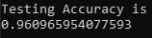
We’ve been able to reach a Test accuracy of 96.06%. A remarkable performance.
Now we’ll plot the confusion matrix to see where the model actually fails.
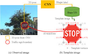
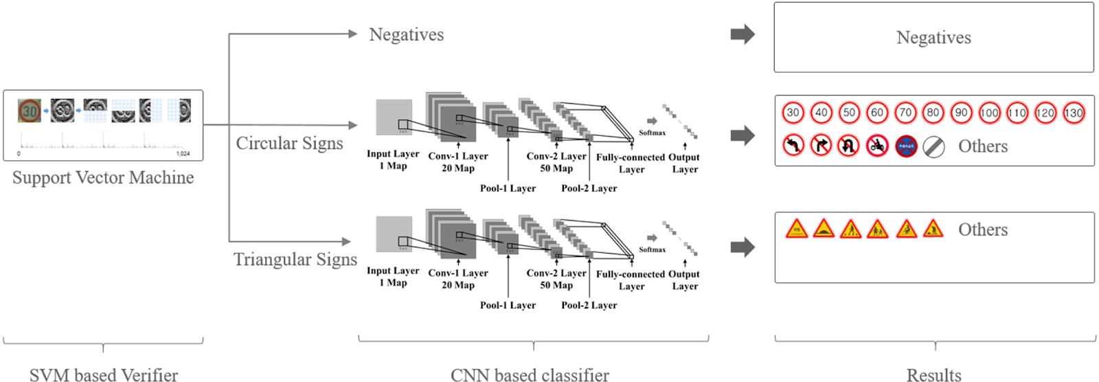
We observe some clusters in the confusion matrix above. It turns out that the various speed limits are sometimes misclassified among themselves. Similarly, traffic signs with traingular shape are misclassified among themselves. We can further improve on the model using hierarchical CNNs to first identify broader groups (like speed signs) and then have CNNs to classify finer features (such as the actual speed limit).
Step 6: Testing the Model on New Images
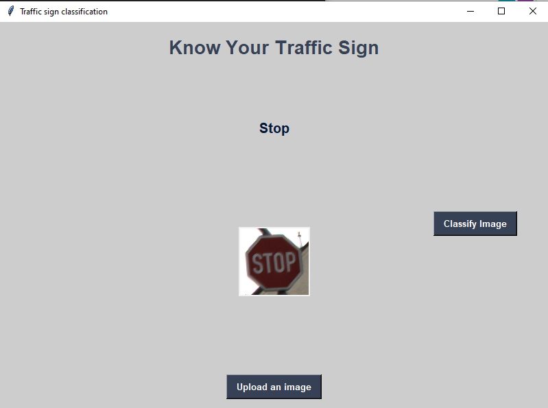
In this step, we will use the model to predict traffic signs type of 5 random images of German traffic signs from the web our model’s performance on these images.
Number of new testing examples: 5
These test images include some easy to predict signs, and other signs are considered hard for the model to predict.
For instance, we have easy to predict signs like the “Stop” and the “No entry”. The two signs are clear and belong to classes where the model can predict with high accuracy.
On the other hand, we have signs belong to classes where has poor accuracy, like the “Speed limit” sign, because as stated above it turns out that the various speed limits are sometimes misclassified among themselves, and the “Pedestrians” sign, because traffic signs with traingular shape are misclassified among themselves.
As we can notice from the top 5 softmax probabilities, the model has very high confidence (100%) when it comes to predict simple signs, like the “Stop” and the “No entry” sign, and even high confidence when predicting simple triangular signs in a very clear image, like the “Yield” sign.
On the other hand, the model’s confidence slightly reduces with more complex triangular sign in a “pretty noisy” image, in the “Pedestrian” sign image, we have a triangular sign with a shape inside it, and the images copyrights adds some noise to the image, the model was able to predict the true class, but with 80% confidence.
And in the “Speed limit” sign, we can observe that the model accurately predicted that it’s a “Speed limit” sign, but was somehow confused between the different speed limits. However, it predicted the true class at the end.
The VGGNet model was able to predict the right class for each of the 5 new test images. Test Accuracy = 100.0%.
In all cases, the model was very certain (80% – 100%).
If you are interested in writing or contributing to formulas, please pay attention to the Writing Formula Section.
If you want to use this formula, please pay attention to the FORMULA file and/or git tag,
which contains the currently released version. This formula is versioned according to Semantic Versioning.
pre-commit is configured for this formula, which you may optionally use to ease the steps involved in submitting your changes.
First install the pre-commit package manager using the appropriate method, then run bin/install-hooks and
now pre-commit will run automatically on each git commit.
$ bin/install-hooks
pre-commit installed at .git/hooks/pre-commit
pre-commit installed at .git/hooks/commit-msg
this state will undo everything performed in the carbon-relay-ng meta-state in reverse order, i.e.
stops the service,
removes the configuration file and
then uninstalls the package.
h5mapper is a pythonic ORM-like tool for reading and writing HDF5 data.
It is built on top of h5py and lets you define types of .h5 files as python classes which you can then easily create from raw sources (e.g. files, urls…), serve (use as Dataset for a Dataloader),
or dynamically populate (logs, checkpoints of an experiment).
h5mapper is on pypi, to install it, one only needs to
pip install h5mapper
developer install
for playing around with the internals of the package, a good solution is to first
git clone https://github.com/ktonal/h5mapper.git
and then
pip install -e h5mapper/
which installs the repo in editable mode.
Quickstart
TypedFile
h5m assumes that you want to store collections of contiguous arrays in single datasets and that you want several such concatenated datasets in a file.
Thus, TypedFile allows you to create and read files that maintain a 2-d reference system, where contiguous arrays are stored within features and indexed by their source’s id.
where the entries correspond to the shapes of arrays or their absence (None).
Note that this is a different approach than storing each file or image in a separate dataset.
In this case, there would be an h5py.Dataset located at data/images/planes/01.jpeg although in our
example, the only dataset is at data/images/ and one of its regions is indexed by the id "planes/01.jpeg"
For interacting with files that follow this particular structure, simply define a class
now, create an instance, load data from files through parallel jobs and add data on the fly :
# create instance from raw sourcesexp=Experiment.create("experiment.h5",
# those are then used as ids :sources=["planes/01.jpeg", "planes/02.jpeg"],
n_workers=8)
...
# add id <-> data on the fly :exp.logs.add("train", dict(loss=losses_array))
get, refs and __getitem__
There are 3 main options to read data from a TypedFile or one of its Proxy
1/ By their id
>>exp.logs.get("train")
Out: {"loss": np.array([...])}
# which, in this case, is equivalent to >>exp.logs["train"]
Out: {"loss": np.array([...])}
# because `exp.logs` is a Group and Groups only support id-based indexing
2/ By the index of their ids through their refs attribute :
Note that, in this last case, you are indexing into the concatenation of all sub-arrays along their first axis.
The same interface is also implemented for set(source, data) and __setitem__
Feature
h5m exposes a class that helps you configure the behaviour of your TypedFile classes and the properties of the .h5 they create.
the Feature class helps you define :
how sources’ ids are loaded into arrays (feature.load(source))
which types of files are supported
how the data is stored by h5py (compression, chunks)
which extraction parameters need to be stored with the data (e.g. sample rate of audio files)
custom-methods relevant to this kind of data
Once you defined a Feature class, attach it to the class dict of a TypedFile, that’s it!
For example :
importh5mapperash5mclassMyFeature(h5m.Feature):
# only sources matching this pattern will be passed to load(...)__re__=r".special$"# args for the h5py.Dataset__ds_kwargs__=dict(compression='lzf', chunks=(1, 350))
def__init__(self, my_extraction_param=0):
self.my_extraction_param=my_extraction_param@propertydefattrs(self):
# those are then written in the h5py.Group.attrsreturn {"p": self.my_extraction_param}
defload(self, source):
"""your method to get an np.ndarray or a dict thereof from a path, an url, whatever sources you have..."""returndatadefplot(self, data):
"""custom plotting method for this kind of data"""# ...# attach itclassData(h5m.TypedFile):
feat=MyFeature(47)
# load sources...f=Data.create(....)
# read your data through __getitem__ batch=f.feat[4:8]
# access your method f.feat.plot(batch)
# modify the file through __setitem__f.feat[4:8] =batch**2
for more examples, checkout h5mapper/h5mapper/features.py.
serve
Primarly designed with pytorch users in mind, h5m plays very nicely with the Dataset class :
TypedFile even have a method that takes the Dataloader args and a batch object filled with BatchItems and returns
a Dataloader that will yield such batch objects.
This project is an implementation of the Unified Diagnostic Services (UDS) protocol defined by ISO-14229 written in Python 3. The code is published under MIT license on GitHub (pylessard/python-udsoncan).
importSomeLib.SomeCar.SomeModelasMyCarimportudsoncanimportisotpfromudsoncan.connectionsimportIsoTPSocketConnectionfromudsoncan.clientimportClientfromudsoncan.exceptionsimport*fromudsoncan.servicesimport*udsoncan.setup_logging()
conn=IsoTPSocketConnection('can0', isotp.Address(isotp.AddressingMode.Normal_11bits, rxid=0x123, txid=0x456))
withClient(conn, request_timeout=2, config=MyCar.config) asclient:
try:
client.change_session(DiagnosticSessionControl.Session.extendedDiagnosticSession) # integer with value of 3client.unlock_security_access(MyCar.debug_level) # Fictive security level. Integer coming from fictive lib, let's say its value is 5client.write_data_by_identifier(udsoncan.DataIdentifier.VIN, 'ABC123456789') # Standard ID for VIN is 0xF190. Codec is set in the client configurationprint('Vehicle Identification Number successfully changed.')
client.ecu_reset(ECUReset.ResetType.hardReset) # HardReset = 0x01exceptNegativeResponseExceptionase:
print('Server refused our request for service %s with code "%s" (0x%02x)'% (e.response.service.get_name(), e.response.code_name, e.response.code))
except (InvalidResponseException, UnexpectedResponseException) ase:
print('Server sent an invalid payload : %s'%e.response.original_payload)
I have a long trajectory of testing out different “Money Manager Apps”, all had one little problem: its usage on other devices.
So I stepped up to the challange to create MY version of a Money Manager App, which would sync with an existing cloud service so I can access my data on any computer I had access to.
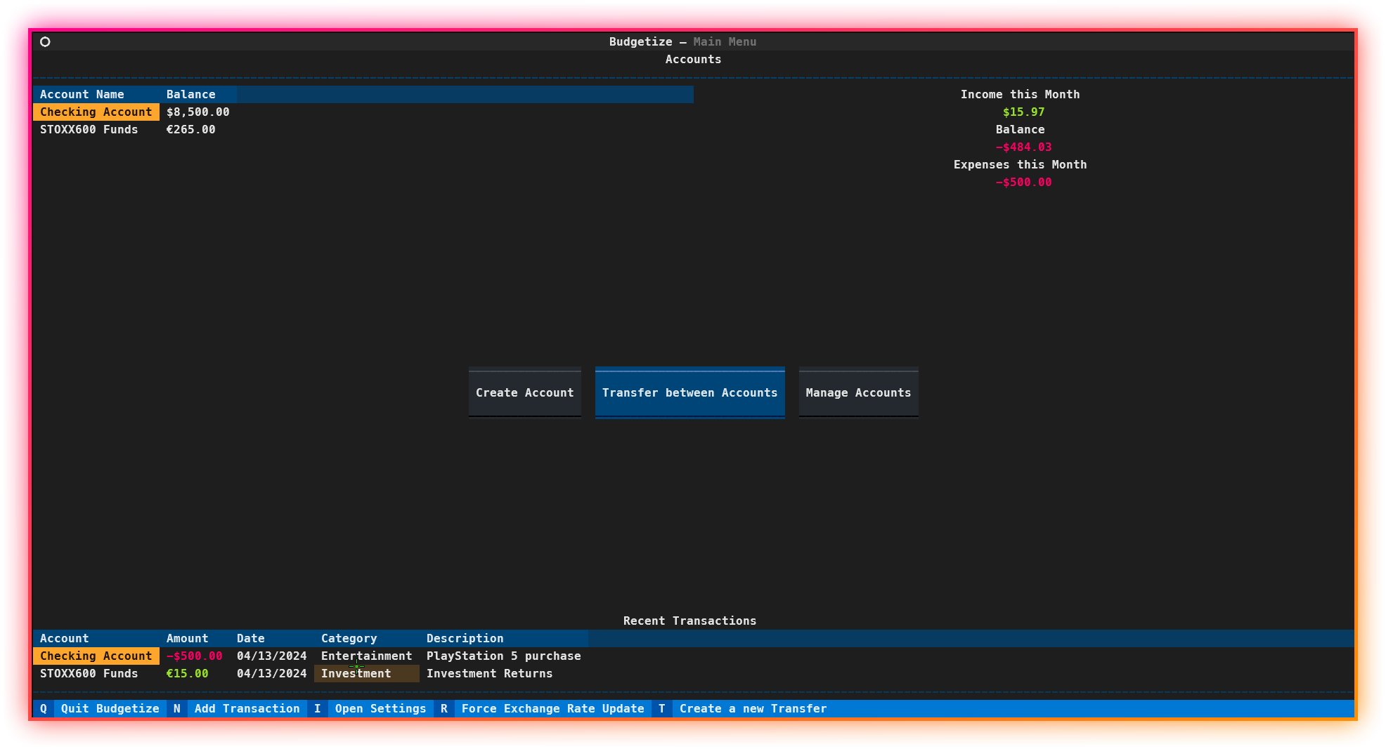
I saw that this wasn’t a UNIQUE idea but it was very useful. So I decided to launch it as an open source project. Although there is still no support with it, Budgetize aims to be a simple and lightweight Money Manager app that sync with the cloud so you can store your data safely and access it anywhere.
I’ll add support in the future to sync your finances with Google Drive by providing an API key yourself.
The compiled version will already be shipped with an existing API key to be ready to use.
🗺 Roadmap
You may check the project’s roadmap in the open projects. Go To Projects
I have a long trajectory of testing out different “Money Manager Apps”, all had one little problem: its usage on other devices.
So I stepped up to the challange to create MY version of a Money Manager App, which would sync with an existing cloud service so I can access my data on any computer I had access to.
I saw that this wasn’t a UNIQUE idea but it was very useful. So I decided to launch it as an open source project. Although there is still no support with it, Budgetize aims to be a simple and lightweight Money Manager app that sync with the cloud so you can store your data safely and access it anywhere.
I’ll add support in the future to sync your finances with Google Drive by providing an API key yourself.
The compiled version will already be shipped with an existing API key to be ready to use.
🗺 Roadmap
You may check the project’s roadmap in the open projects. Go To Projects
A lumo based test runner for selenium-webdriver using node-js bindings
and clojurescript
Motivation
I wanted to play with the node-js bindings for selenium-webdriver, and
have used lumo with success in the past to leverage npm via
clojurescript.
The clojure libraries I’ve seen that integrate with selenium have
focused on providing api functions, either through reflection or
direct specification, so that you have access to them in an idiomatic
way.
Though this is useful, I didn’t want to create a bindings library, and
instead wanted to focus on direct interop to discover useful patterns,
and then capture those patterns and allow them to be leveraged as
interpreted data.
The poe.core/interpret multimethod provides a way to capture these
patterns.
The node bindings present an interesting interface for clojure,
because most operations are performed by chaining promises together to
create the sequence of events to test. This was another area that I
thought could be simplified for test specification.
The poe.core/run function captures a way for a vector of operations
to be used to define and run a test, handling all of the chaining for
you.
Install
This library depends on selenium-webdriver, and is scoped to expect
the use of chromedriver to operate with google chrome. Not currently
planning to go for more support, unless it becomes important to.
Also, I’m assuming OSX with brew, if you aren’t using this, you can
get the dependencies some other way.
This project includes tools to build portable images of a Python shell (powered by xonsh and with xxh support) destinated to be used for pentesting and bug bounties (among others, ethical, hacking purposes).
It includes an easy way to build custom appimages with a portable shell (that could be run in Linux, Unix, Windows and others OS without any trouble) that supports Python sintax and may include additional toosl.
This image is intended to be used along with xxh proyect so you could extend it’s functionality through the network using ssh connections. For example: you could connect to an old Solaris machine using xxh and easily run your portable image with all your plugins, configurations and additionally installed tools.
xxh – Bring your favorite shell wherever you go through the ssh.
Compatible with
Wazuh – The Open Source Security Platform: Wazuh is a tool that can be used to gather, decode and analyze logs. Offshell can be integrated with Wazuh by sending the logs generated by our history backend plugin to Wazuh to be analyzed and indexed into a search engine such as Elasticsearch (or OpenSearch, soon). Also, Wazuh can analyze the received logs and generate alerts based on some pre-defined rules for interesting security events such as detected vulnerabilities or privilege escalations.
Getting Started
Installation of official images.
Important: the appimage requires Git to properly work!
We have some pre-built images available here at Github.
It is not required to install Xonsh, you only need to download the last built appimage and make it executable to run the shell.
After adding that block to your ossec.conf file, if you agent is correctly connected to a Wazuh manager it woud start sending information about exeuted commands to your server and it will index it to a Elasticsearch index.
You can modify this proyect and build your own appimages using the tools included in the build_appimage directory.
For example, to include more python depedencies in the appimage you only need to modify the pre-requirements.txt file.
You could also modify the xonsh/xxh configuration file to add functionalities, plugins, aliases, etc..
Roadmap
See the open issues for a list of proposed features (and known issues).
Contributing
Contributions are what make the open source community such an amazing place to be learn, inspire, and create. Any contributions you make are greatly appreciated.
Fork the Project
Create your Feature Branch (git checkout -b feature/AmazingFeature)
Commit your Changes (git commit -m 'Add some AmazingFeature')
Push to the Branch (git push origin feature/AmazingFeature)
Open a Pull Request
License
Distributed under the GLP3 License. See LICENSE for more information.


.png)
.png)


.png)
.png)