


epanetReader is an R package for reading water network simulation data in Epanet’s .inp and .rpt formats into R. Some basic summary information and plots are also provided.
Epanet is a highly popular tool for water network simulation. But, it can be difficult to access network information for subsequent analysis and visualization. This is a real strength of R however, and there many tools already existing in R to support analysis and visualization.
In addition to this README page, information about epanetReader is available from Environmental Modelling & Software (pdf) and ASCE Conference Proceedings (pdf).
- the latest released version: install.packages(“epanetReader”)
- the development version: devtools::install_github(“bradleyjeck/epanetReader”)
Read network information from an .inp file with a similar syntax as the popular read.table or read.csv functions. Note that the example network one that ships with Epanet causes a warning. The warning is just a reminder of how R deals with integer IDs.
library(epanetReader)
n1 <- read.inp("Net1.inp")
## Warning in PATTERNS(allLines): patterns have integer IDs, see ?epanet.inp
## Warning in CURVES(allLines): curves have integer IDs, see ?epanet.inp
Retrieve summary information about the network.
summary(n1)## EPANET Example Network 1
## A simple example of modeling chlorine decay. Both bulk and
## wall reactions are included.
##
## Number
## Junctions 9
## Tanks 1
## Reservoirs 1
## Pipes 12
## Pumps 1
## Quality 11
## Coordinates 11
## Labels 3
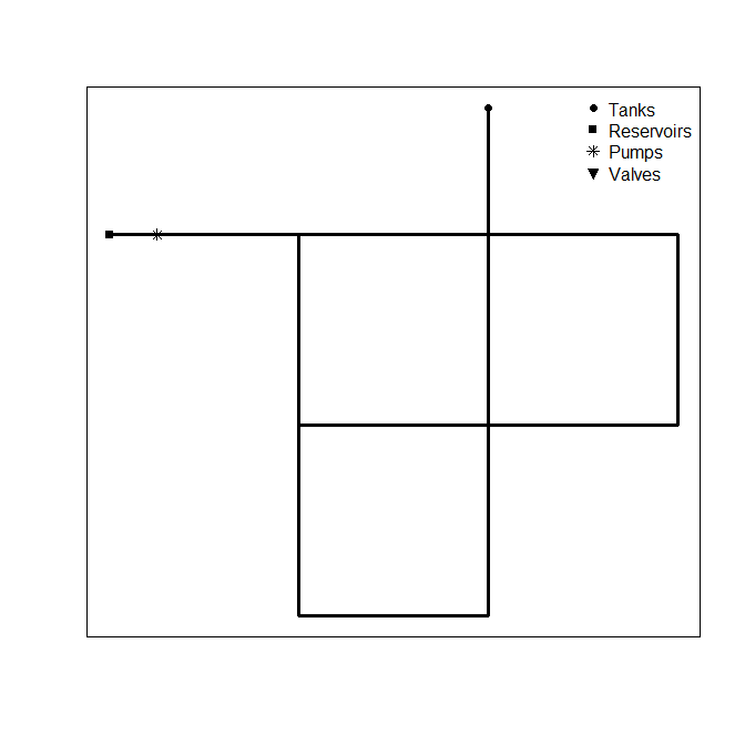
A basic network plot is also available
plot(n1)
The read.inp function returns an object with structure similar to the .inp file itself. A section in the .inp file corresponds to a named entry in the list. These entries are accessed using the $ syntax of R.
names(n1)## [1] "Title" "Junctions" "Tanks" "Reservoirs" "Pipes"
## [6] "Pumps" "Valves" "Demands" "Patterns" "Curves"
## [11] "Controls" "Rules" "Energy" "Status" "Emitters"
## [16] "Quality" "Sources" "Reactions" "Mixing" "Times"
## [21] "Report" "Options" "Coordinates" "Vertices" "Labels"
## [26] "Backdrop" "Tags"
Sections of the .inp file are stored as a data.frame or character vector. For example, the junction table is stored as a data.frame and retrieved as follows. In this case patterns were not specified in the junction table and so are marked NA.
n1$Junctions## ID Elevation Demand Pattern
## 1 10 710 0 NA
## 2 11 710 150 NA
## 3 12 700 150 NA
## 4 13 695 100 NA
## 5 21 700 150 NA
## 6 22 695 200 NA
## 7 23 690 150 NA
## 8 31 700 100 NA
## 9 32 710 100 NA
A summary of the junction table shows that Net1.inp has nine junctions with elevations ranging from 690 to 710 and demands ranging from 0 to 200. Note that the node ID is stored as a character rather than an integer or factor.
summary(n1$Junctions)## ID Elevation Demand Pattern
## Length:9 Min. :690.0 Min. : 0.0 Mode:logical
## Class :character 1st Qu.:695.0 1st Qu.:100.0 NA's:9
## Mode :character Median :700.0 Median :150.0
## Mean :701.1 Mean :122.2
## 3rd Qu.:710.0 3rd Qu.:150.0
## Max. :710.0 Max. :200.0
Results of the network simulation specified in Net.inp may be stored in Net1.rpt by running Epanet from the command line. Note that the report section of the .inp file should contain the following lines in order to generate output readable by this package.
[REPORT]
Page 0
Links All
Nodes All
On windows, calling the epanet executable epanet2d runs the simulation.
>epanet2d Net1.inp Net1.rpt

... EPANET Version 2.0

  o Retrieving network data
  o Computing hydraulics
  o Computing water quality
  o Writing output report to Net1.rpt

... EPANET completed.
The .rpt file generated by Epanet may be read into R using read.rpt(). The simulation is summarized over junctions, tanks and pipes.
n1r <- read.rpt("Net1.rpt")
summary(n1r)
## Contains node results for 25 time steps
##
## Summary of Junction Results:
## Demand Pressure Chlorine
## Min. : 0.0 Min. :106.8 Min. :0.1500
## 1st Qu.: 80.0 1st Qu.:116.1 1st Qu.:0.3500
## Median :120.0 Median :119.8 Median :0.5100
## Mean :122.2 Mean :119.6 Mean :0.5434
## 3rd Qu.:160.0 3rd Qu.:123.0 3rd Qu.:0.7400
## Max. :320.0 Max. :133.9 Max. :1.0000
##
## Summary of Tank Results:
## Demand Pressure Chlorine
## Min. :-1100.000 Min. :48.22 Min. :0.590
## 1st Qu.: -660.000 1st Qu.:52.00 1st Qu.:0.660
## Median : 258.000 Median :55.52 Median :0.750
## Mean : -5.741 Mean :54.86 Mean :0.764
## 3rd Qu.: 505.380 3rd Qu.:57.54 3rd Qu.:0.850
## Max. : 1029.420 Max. :60.04 Max. :1.000
##
## Contains link results for 25 time steps
##
## Summary of Pipe Results:
## Flow Velocity Headloss
## Min. :-1029.42 Min. :0.0000 Min. :0.000
## 1st Qu.: 41.37 1st Qu.:0.3475 1st Qu.:0.110
## Median : 113.08 Median :0.5700 Median :0.300
## Mean : 245.35 Mean :0.8070 Mean :0.644
## 3rd Qu.: 237.23 3rd Qu.:1.0075 3rd Qu.:0.755
## Max. : 1909.42 Max. :2.7300 Max. :3.210
##
## Energy Usage:
## Pump usageFactor avgEfficiency kWh_per_Mgal avg_kW peak_kW dailyCost
## 1 9 57.71 75 880.42 96.25 96.71 0
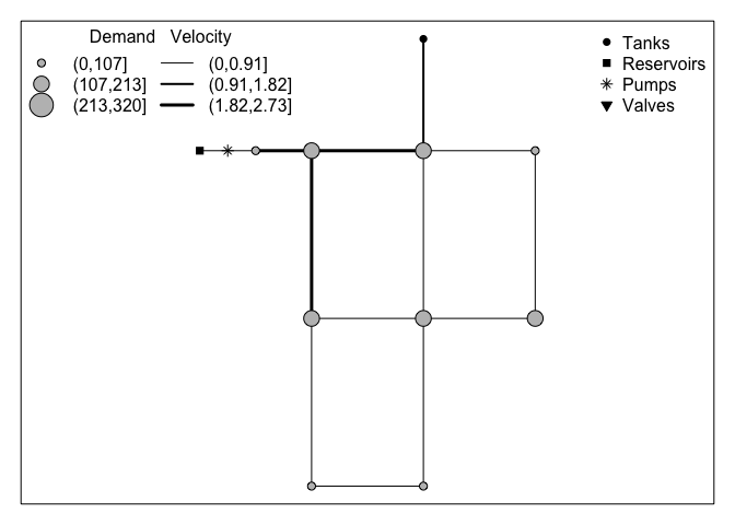
The default plot of simulation results is a map for time period 00:00:00. Note that the object created from the .inp file is a required argument to make the plot.
plot( n1r, n1)
In contrast to the treatment of .inp files described above, data from .rpt files is stored using a slightly different structure than the .rpt file. The function returns an object (list) with a data.frame for node results and data.frame for link results. These two data frames contain results from all the time periods. This storage choice was made to facilitate time series plots.
Entries in the epanet.rpt object (list) created by read.rpt() are found using the names() function.
names(n1r)## [1] "nodeResults" "linkResults" "energyUsage"
Results for a chosen time period can be retrieved using the subset function.
subset(n1r$nodeResults, Timestamp == "0:00:00")## ID Demand Head Pressure Chlorine note Timestamp timeInSeconds
## 1 10 0.00 1004.35 127.54 0.5 0:00:00 0
## 2 11 150.00 985.23 119.26 0.5 0:00:00 0
## 3 12 150.00 970.07 117.02 0.5 0:00:00 0
## 4 13 100.00 968.87 118.67 0.5 0:00:00 0
## 5 21 150.00 971.55 117.66 0.5 0:00:00 0
## 6 22 200.00 969.08 118.76 0.5 0:00:00 0
## 7 23 150.00 968.65 120.74 0.5 0:00:00 0
## 8 31 100.00 967.39 115.86 0.5 0:00:00 0
## 9 32 100.00 965.69 110.79 0.5 0:00:00 0
## 10 9 -1866.18 800.00 0.00 1.0 Reservoir 0:00:00 0
## 11 2 766.18 970.00 52.00 1.0 Tank 0:00:00 0
## nodeType
## 1 Junction
## 2 Junction
## 3 Junction
## 4 Junction
## 5 Junction
## 6 Junction
## 7 Junction
## 8 Junction
## 9 Junction
## 10 Reservoir
## 11 Tank
A comparison with the corresponding entry of the .rpt file, shown below for reference, shows that four columns have been added to the table. These pieces of extra info make visualizing the results easier.
  Node Results at 0:00:00 hrs:
  --------------------------------------------------------
                     Demand      Head  Pressure  Chlorine
  Node                  gpm        ft       psi      mg/L
  --------------------------------------------------------
  10                   0.00   1004.35    127.54      0.50
  11                 150.00    985.23    119.26      0.50
  12                 150.00    970.07    117.02      0.50
  13                 100.00    968.87    118.67      0.50
  21                 150.00    971.55    117.66      0.50
  22                 200.00    969.08    118.76      0.50
  23                 150.00    968.65    120.74      0.50
  31                 100.00    967.39    115.86      0.50
  32                 100.00    965.69    110.79      0.50
  9                -1866.18    800.00      0.00      1.00  Reservoir
  2                  766.18    970.00     52.00      1.00  Tank
Results of a multi-species simulation by Epanet-msx can be read as well.
The read.msxrpt() function creates an s3 object of class epanetmsx.rpt. Similar to the approach above, there is a data frame for node results and link results.
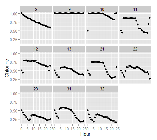
The ggplot2 package makes it easy to create complex graphics by allowing users to describe the plot in terms of the data. Continuing the Net1 example Here we plot chlorine concentration over time at each node in the network.
library(ggplot2)
qplot( data= n1r$nodeResults,
       x = timeInSeconds/3600, y = Chlorine,
facets = ~ID, xlab = "Hour") 
The animation package is useful for creating a video from successive plots.
# example with animation package
library(animation)

#unique time stamps
ts <- unique((n1r$nodeResults$Timestamp))
imax <- length(ts)

# generate animation of plots at each time step
saveHTML(
  for( i in 1:imax){
    plot(n1r, n1, Timestep = ts[i])
  }
)Rossman, L. A. (2000) Epanet 2 users manual. US EPA, Cincinnati, Ohio.
 https://github.com/bradleyjeck/epanetReader